Contents:
Download the source code , and save it as atv.pro in a directory that's listed in your IDL path. You'll also need to install a few IDL libraries into your IDL path: these include the IDL Astronomy User's Library, the Coyote Graphics Library, and Craig Markwardt's cmps_form.pro routine. See the ATV main page for links to these libraries. To read fpack-compressed fits files you'll also need to have the CFITSIO library and fpack/funpack routines installed (these are not IDL routines).
Important for Mac users: you
need to issue the command "device, retain=2" before starting ATV
in order for color map updates to work properly. This isn't
included in ATV itself since there may be other situations where
this command wouldn't be desired, but with recent updates to MacOS
(El Capitan), ATV will not function properly without this. This
command basically tells the window manager to store window
contents so they can be redisplayed quickly. I put this command in
my IDL startup file so that it gets executed at the start of each
IDL session. In the next release, I'll update this so that
ATV automatically detects whether it's running on a mac, and then
issues the retain command if necessary.
Once everything is installed, just start IDL, and type atv.
To display an array that's in memory, just pass its name to atv like this:
atv, array_name [,header = head]
[,min = min_value] [,max=max_value] [,/linear] [,/log] [,/histeq]
[,/asinh] [,/align] [,/stretch] [,/block]
Similarly, to display a fits file, you can pass the file name to atv:
atv, 'fitsfile_name' [,
options...]
The command-line options are:
ATV can recognize a variety of
fits image types:
The routine uses xmanager to ensure that an IDL session can have only one atv window running at a time, so if you already have an atv running and you type "atv, array_name", the display comes up in your previously existing atv window.
Note: all coordinates are IDL-based, which means that a 1024x1024 array will have element (0,0) at the lower left and (1023,1023) at the upper right corner. Remember this when comparing with pixel coordinates in IRAF or SAOimage, where arrays start with element 1 instead of element 0.
How to change the ATV window orientation.Tips on IDL settings for color maps and windows.
ATV works in 8-bit, 16-bit, or
24-bit color. When ATV was first written, 8-bit color
was the norm, but now most computers will be using 24-bit
color. IDL handles color tables very differently for these
two cases. For 24-bit color, most users will be using 24-bit true
color mode.
I usually run IDL in 24-bit color (using Linux or Mac OS X), and I use the following commands in my IDL startup file:
device, true_color = 24

        device, decomposed = 0

        device, retain = 2
On MacOS, as of Yosemite or El
Capitan, the "retain=2" command is absolutely necessary or else
ATV is unusable, so ATV now issues this command if it is running
on MacOS.
As of version 3.0, ATV is now
using the Coyote
Graphics
library for plotting instead of the basic IDL commands like
tv or plot. This has two major advantages: it works
identically in decomposed=0 or decomposed=1 mode, and it enables
the use of named colors in plots (like color="red") regardless of
which color table is currently being used. So, now it's no
longer necessary to specify "device, decomposed=0" to use ATV.
How to change the image scaling.
When you read a new image into
ATV, it is auto-scaled by default. If you'd rather have the
default setting be to display an image with its full intensity
range, then go into the ATV code to the subroutine
atv_initcommon.pro, and change the definition of the state
variable default_autoscale to 0.
The default setting is now asinh
scaling, since this works really well. The asinh scaling
uses an adjustable parameter beta. Typically you want beta
to be about equal to the standard deviation of the count level in
background sky pixels. When you read in a new image, ATV
calculates the sky mode and sky sigma automatically, and uses
those values to determine the autoscaling and beta
parameters. If you want to change beta, go to the Scaling
menu and select "Asinh Settings".
The autoscaling parameters are
different depending on whether your image is displayed in linear,
log, histeq, or asinh stretch. Just play around with it to
get a feeling for what it does. Autoscaling sets the "min"
value to be the sky mode minus 2 times the sky sigma. The
"max" value is set to be either the sky mode plus n times the
image standard deviation (n=2 for linear and n=4 for log scaling),
or the maximum pixel value in the image (asinh or histeq scaling).
Once an image has been displayed, there are a few ways to change the data range that gets mapped into the color table:
Once a scaling option
(log/linear/histeq/asinh) is chosen, it remains in effect until a
new scaling option is selected.
If you prefer to have linear or
log scaling as the default instead of asinh, go into the routine
atv_initcommon and change the initial value of the scaling
variable in the main state structure. On extremely
large images, the asinh scaling can take noticeably longer to run,
so if you don't like waiting for it, going to log or linear
stretch will help new images to load in more quickly.
How to change the color tables and stretch.
The ColorMap menu offers a
choice of several color tables. A new addition in version
3.0 is the cubehelix
color map. The cubehelix color map has the nice feature that the
color table entries increase smoothly in brightness while also
constantly varying in hue. If you select "Cubehelix
Settings" from the ColorMap menu, you'll get a widget that lets
you modify the four parameters of the cubehelix color map so you
can design your own color table.
To invert the color table, just click on the "Invert" button.
Brightness and contrast can be modified by setting MouseMode to "Color", and then by dragging the mouse over the main image window with mouse button 1 held down. Moving the mouse horizontally changes brightness, and moving vertically changes contrast. The color bar next to the panning window shows the current color table.
While in Color mode, you can use mouse button 2 or 3 to recenter the image on the current cursor position.
What does the restretch button do?
When you click the restretch
button, the brightness and contrast are reset back to their
default values, to linearize the color table. At the same
time, the min and max values are adjusted to preserve the
appearance of the image as closely as possible. This can be
useful if you're viewing an image with a very hard stretch (i.e.
high contrast) and you want to have more dynamic range in the
color table while keeping the overall appearance of the display
similar. Restretch works best for images displayed with a
linear scaling.
The restretch feature doesn't
always do exactly what you expect if you're using asinh or log
scaling, because it's not always possible to preserve the exact
appearance of the image when restretching. In histeq mode,
the restretch button doesn't do anything.
How to zoom in and out, and look at different portions of the image.
To zoom in or out, while preserving the current central pixel of the display, click on "ZoomIn" or "ZoomOut". To set the zoom level back to the default (1 display pixel = 1 data pixel), click on "Zoom1". To center the image on the display viewport, click on "Center".
When MouseMode is set to "Zoom", the mouse buttons can also control zooming and centering:
Another way to zoom in or out is
to use the - or + key on the keyboard, with the cursor in the main
draw window. You can also zoom in by pressing the = key,
which saves you the trouble of having to hit the shift key to type
+.
While the cursor is in the main
display window, the ATV status bar shows the x and y coordinates
of the cursor and the data value at that pixel. To move by
one pixel at a time, you can use either the arrow keys or your
numeric keypad (with "NumLock" turned on). You can move up,
down, left, right, or diagonally.
When the mouse mode is set to
"Color", you can use button 2 or 3 to center the image on the
current pixel.
How to blink 2 images against each other.
Load in the first image, and get
the display exactly how you want it. Then, go to the Blink
menu and select "SetBlink1". Then load in the second image
and set MouseMode to "Blink". Now, with the cursor in the
main draw window, just hold down the first mouse button to display
the first image, and release the button to show the current
image. You can save up to 3 blink images and blink them with
mouse buttons 1, 2, or 3. If you have fewer than 3 mouse
buttons, you won't be able to use all 3 blink images.
You can also set the blink
images with keyboard events, using shift-1, shift-2, and
shift-3. In other words, type "!" for SetBlink1, "@" for
SetBlink2, and "#" for SetBlink3.
How to make an RGB color image.
ATV can make RGB "true-color"
images in a rudimentary way. To do this, first set the
colormap to grayscale, and don't invert the colormap. Load
your "R" image and get the color stretch just the way you want it,
and then save it in blink channel 1 with "SetBlink1". Do the
same for your G image in blink channel 2 and your B image in blink
channel 3. Then, just select "Blink->MakeRGB" and ATV
will make a truecolor RGB image using the 3 blink channels.
The color image is not adjustable in any way: if you want to
change the color balance, the only way to adjust it is to re-load
in your original images, change the color stretch, and then save
them to the blink channels again.
If you like how your RGB image
came out, you can save it to a file using "File->WriteImage" to
save it to a jpg, png, or tiff image. Here's an example.
The RGB image will stay in the
ATV display window until you do anything that changes the display
settings, like zooming or changing the color stretch. As
soon as you do that, ATV goes back to its normal display mode with
the last image that was loaded.
How to select the coordinate system.
If the image header has a valid world coordinate system (WCS), then ATV will display the coordinates of the cursor position. By default, it uses the native coordinate system and equinox given in the image header. ATV can also convert the native coordinates into J2000, B1950, ecliptic, or galactic coordinates. To change the output to a different system, go to the ImageInfo menu and select one of the coordinate options.
If you're viewing a 2-d
spectroscopic image with a wavelength solution, then ATV will
display the wavelength at the cursor position. So far, I've
only tried this for HST STIS images, so I don't know if it will
work for other data types.
From the File menu, pull down
"WriteFits", "WriteImage", or "WriteEPS".
The WriteFits selection gives
you the option to write out a fits image of the current main
display image. If you've read in an image and then rotated
or flipped it, this will write out the rotated or flipped version
of the image. It will write out the header information into
the
image.
The WriteImage menu gives you
the option to write out a PNG, JPG, or TIFF image of the current
display, pretty much exactly as you see it on screen.
For postscript output, the postscript file paramters are set in a window that brings up Craig Markwardt's cmps_form widget. This window is fairly self-explanatory, but take a look here if you need more information, or look at the cmps_form.pro source. One important point is that if the postscript options are set to black and white (i.e. color=off in the postscript widget form), then the postscript device will not pay any attention to color maps at all, and the resulting color map in the postscript file will be just a linear B-W scale regardless of the color stretch in the ATV window. So it's usually best to leave color on in the ps parameters window.
For postscript output, the program will by default put a black frame around the image border. To disable this, edit the atv.pro source and in the routine atv_initcommon, change the definition of state.frame to 0.
One other note about postscript
output: the atv_writeps routine uses scaleable pixels in creating
the ps image, so it can't handle fractional pixels at the edge of
the viewport. So, in postscript output, any fractional
pixels at the edges of the display image will be included as
complete pixels in the ps image. The result is that for a
highly zoomed image, the postscript output file may have a
slightly different size than the screen image. This will
only be noticeable when you've zoomed in to make the pixels really
big on screen. The advantage of doing things this way is
that it makes the postscript files far more compact for highly
zoomed images. On the other hand, for really big images
which are zoomed "out" to fit the whole image in the display
viewport, the size of the postscript output file can be pretty
huge, since the full resolution of the original image is included
in the postscript file.
If you want to create image
output in png or jpg format for use on a web page or something
like that, you can sometimes get better results if you create a
postscript file, and then use the ImageMagick
"convert" program to convert to png, instead of having atv create
a png file directly. This can make a noticeable difference
if you have any overplots on your image. When atv creates a
png or jpg output image, it creates a pixel-by-pixel copy of
what's in the main display window, but for postscript output it
creates higher-resolution scaleable output. The two pictures
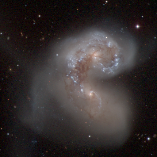
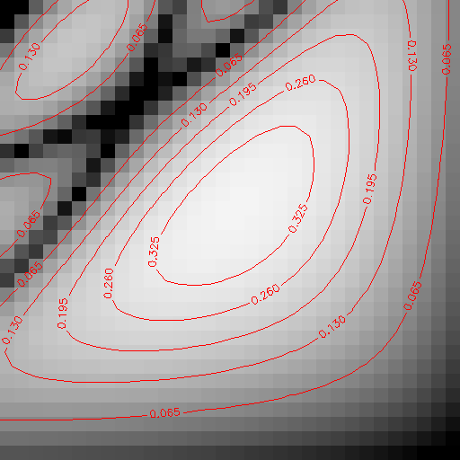
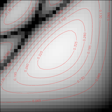
below show an example, with contour overplots on top of an
image. The picture on the left shows the result from using
atv's WriteImage feature to create a png image directly. The
second picture shows the result from using WritePS to create a
postscript image, and then using ImageMagick to convert the
postscript to png (with the command convert image.ps image.png).
In the converted image, you can see that ImageMagick has used
antialiasing on the contour lines and fonts and this gives a nicer
looking result. You can also convert postscript to png or
jpg using the Apple Preview program.
|
|
Just grab a corner of the atv window with your mouse, and drag it to the desired size. The image will redisplay, preserving the central pixel of the display viewport. Note: the code is set to have a minimum window size, so if you try to make the atv window really small it will set itself to this minimum size.
If you resize the main window
and it comes out funny, just grab the corner and move it a little
bit- that usually fixes the problem.
How to do quick aperture photometry.
Position the cursor right on top of the object you want to measure, and hit "p". This brings up the photometry widget window. The window displays the cursor position, computed object centroid, sky level, and number of counts in the aperture. By changing the text in the input boxes, you can modify the centering box size, the photometric aperture radius, and the inner and outer sky radii. Be sure to hit "Return" after changing one of these numbers, otherwise they won't be input into the photometry routines. To measure a new object, just move the cursor on top of the object and hit "p" again.
ATV will try to find the centroid of the nearest object to the cursor position when doing photometry. If it's not finding the object properly, you can tweak the centering box size. If you want to do photometry at the current cursor position without recentering on the nearest object, set the centerbox size to 0. Please note that if you do this, your aperture will always be centered on the middle of the pixel at the current cursor position.
To view the object's radial profile, click on "Show Radial Profile." The FWHM is measured directly from the radial profile, and is not based on a fit to the profile. It's just the radius at which the count level drops to half of its peak value. So this number may come out somewhat different from what you'd get if you did a Gaussian fit to the profile or to the 2-dimensional shape of the object.
You can also set the mouse mode to ImExam, and use mouse button 1 for photometry at the current cursor position. Or, you can bring up the photometry window from the ImageInfo menu.
The routine is set up so that the photometric aperture radius is always forced to be smaller than the inner sky radius, and the inner sky aperture is forced to be smaller than the outer sky aperture.
ATV uses the idlastro library routine "aper" to do the photometry calculations. For details on how the photometry is done, look at the aper code in the idlphot subdirectory of your idlastro distribution. Also, in the idlastro top-level 'text' subdirectory there is a file called daophot.tex that gives further details on the photometry routines. ATV doesn't use daophot to calculate the object centroids, though, because the daophot routine calculates the centroids for all objects in an image, while ATV just wants to look at one object at at time.
If you click on the "Photometry Settings" button, ATV will bring up a dialog box which gives you a few options:
Choice of sky algorithm: Gives
you a choice between using the mode sky value calculated by the
GSFC IDLPhot "sky" routine (this is usually the best), or a simple
median of the pixel values in the sky annulus, or no sky
subtraction. Depending on the image statistics and noise
properties, the IDLPhot sky and median sky may differ
significantly. Look at where the sky level comes out in the
radial profile window to see whether this matters for your
data.
Choice of counts or
magnitudes: If you want output in magnitudes, you can set
the magnitude zeropoint in the dialog box. For
magnitudes to come out right, you need the zeropoint and exposure
time to be set correctly. ATV will attempt to read the
exposure time from the EXPTIME header keyword. If it's not
there, it will assume an exposure time of 1 second, but you can
adjust this in the photometry settings window.
By default, ATV will not return
uncertainties on the photometric measurements. The reason
for this is that the photometry errors will only make sense if the
gain and readout noise are given correctly. It's better to
not calculate any error bars at all, than to calculate meaningless
error bars. The readnoise and gain don't affect the counts
(or magnitude) within the photometric aperture, but they are
necessary to know the correct measurement uncertainty.
You can enter the readnoise and gain values in the photometry
settings window, and then turn on the option to calculate
photometric errors there too. But, make sure that you're
entering the correct values, especially accounting for any scaling
factors that have been applied to your image, or any co-adding or
averaging of frames, that would change the effective values of
gain and readnoise. Don't try to use the photometric errors
unless you know what these numbers really mean for your data!
For standard CCD images, I've
tested the photometry results against IRAF's built-in aperture
photometry routines, and under normal circumstances the results
come out essentially identically, including the error bars.
However, if you're using ATV for photometry, please be aware that
the IDL photometry routines have not been tested as extensively as
other photometry tools such as DAOPHOT or IRAF's photometry
routines.
If you click on the "Write
results to file..." button, it will prompt you for a filename to
save your aperture photometry results. If the file already
exists, it will append the new data to the existing file.
How to do quick-look spectral
extractions.
The spectral extraction feature
is intended primarily for quick-look reductions, and it does not
have the full feature set of a general purpose extraction tool
like apall in IRAF. ATV doesn't (yet) do optimal
extractions, and doesn't allow interactive editing of trace
points. Also, the background is calculated in a very simple
way, just by taking the median value of each background region,
and then averaging the upper and lower background values
together. This could be improved in the future by adding
additional code to do rejection iterations for cosmic rays in the
background region, allowing a polynomial fit to the background,
etc. However, changes like these would require more
adjustable parameters and more user interaction, so for now I've
chosen to just keep things as simple as possible. The
extraction routine should work very well for normal long-slit data
as long as the object is not extremely faint. It can also
work well on multi-slit spectra or echelle spectra (even with
curved spectral orders)- in this case you might have to set the
extraction start and end parameters manually to define the region
to be extracted. However, the background subtraction is just
done column-by-column, so if you have a spectrum where the night
sky lines are tilted or strongly curved, the background
subtraction will not work well.
The extracted spectrum can be
saved either as a FITS spectrum or a plain 2-column ASCII file.
How to view image statistics for a region.
Just hit "i" to bring up the
image statistics window, or set the mouse mode to "ImExam" and use
mouse button 2. The statistics window will show the image
min and max value, and the min, max, mean, and median for a box
centered on the cursor position. You can change the box
center or the box size by entering new numbers in the input
boxes. To see a zoomed-in view of the stats region, click on
"Show Region". The box size has to be odd, so that the
cursor position will be at the center of the box.
You can also bring up the Stats window from the ImageInfo menu.
Go to the ImageInfo menu, and select ImageHeader. If you've read in a fits image that has a valid header, the header will appear in a new window.
How to bring up row and column plots, and surface and contour plots.
With the cursor in the main draw window, the keyboard is used to bring up the plot window.
How to overplot text and graphics on the image.
Overplots are done via IDL command-line routines, or from the "Labels" menu. The commands atvxyouts, atvplot, and atvcontour work just like the standard IDL commands xyouts, plot, and contour. That is, for positioning the labels, you need to specify the actual (x, y) pixel coordinates in the image where you'd like the labels to appear. Here are some examples:
To overplot text on an image:
atvxyouts, 100, 100, 'Your Ad Here', color='green', charsize=2
To overplot a line segment:
atvplot, findgen(50), findgen(50), color='red'
To mark a data point:
atvplot, [100], [100], psym=2
To overplot contour levels:
atv, array_name
atvcontour, array_name, c_colors=['magenta', 'yellow']
You can use the atvcontour command to overplot contours of one image on top of an entirely different image which is already displayed in the main ATV window. This will work best if the two images have the same dimensions, of course.
The atvplot command can be used to overplot any plot symbol on top of a list of image coordinates, similar to the IRAF "tvmark" command.
To erase plot overlays, use atverase. The command "atverase" by itself will remove all plot overlays, and "atverase, n" will erase the most recent n plot overlays. When you display a new image, all plot overlays are erased so they won't plot on the new image.
The atvxyouts, atvplot, and atvcontour commands can take a variety of command-line keywords that let you customize the font, line thickness, line type , and character thickness, and other plot attributes. See the keyword lists for the IDL xyouts, plot, and contour commands for details.
The default color for all overplots is red. The available colors are (going from 0 to 7) black, red, green, blue, cyan, magenta, yellow, and white.
The atvxyouts and atvcontour
commands can also be accessed, with a limited range of options,
from the "Labels" pull-down menu. The "TextLabel" or
"Contour" menu items bring up a dialog box that let you specify
the label characteristics. The "EraseLast" menu item
removes the most recent plot overlay, and "EraseAll" removes all
overplots. With the cursor in the main display window, you
can also hit the 'e' key to erase all overplots.
If your image has a valid world coordinate system in the header, you can display a compass (i.e. arrows pointing north and east) by selecting Compass from the Labels menu. You can also plot a scale bar (i.e. a bar showing the size of 1 arcsecond) by selecting Scalebar from the Labels menu. The compass option uses a GSFC library routine, and the scalebar option uses a slightly modified version of a library routine which allows re-scaling the size of the scale bar depending on the zoom factor.
There's nothing built in to ATV that selects which font family is chosen. You can issue a !p.font command at the IDL prompt to change the font family between postscript, true type, or vector fonts. This is something I'll try to work on in the future, to give the use the option to switch fonts from within ATV. See the IDL online help or manuals for details on how IDL handles fonts.
The new Regions menu allows you
to plot image regions in a way that's modeled after what DS9 and
other image display routines use. You can plot lines, boxes,
circles, and ellipses, with the coordinates and sizes set by
either pixel coordinates or RA,Dec if available. You can
also save your list of region overplots as a file and read it in
later.
Thanks to David Schlegel for
writing the original versions of the subroutines for creating plot
overlays.
How to view
image stacks or cubes.
This is a new feature in version
2.2. If you read in a 3-dimensional FITS file or array, ATV
will attempt to display it by bringing up a new slider widget that
lets you select which slice of the array you want to view.
You can also view the mean or median of a set of slices.
If the array has the form (x, y,
slice) then ATV will display it starting with the (x, y) image
from slice 0. ATV will also try to recognize Keck OSIRIS
reduced data cubes, which are formatted as (y, x, lambda).
For those data cubes, ATV will reformat the array as (x, y,
lambda) and the slider widget will let you choose which wavelength
slice to display.
I'd like to extend this to
support other formats of data cubes from IFU instruments, so if
you find that ATV won't properly display a 3-d data cube from some
other instrument, let me know. If you can send me an example data
file, I can try to work on adding support for it.
If you select the "vector" mouse
mode, you can use the right mouse button to do a "depth plot",
where you select a 2-d region of the image and extract a spectrum
or profile through the data cube within that spatial region.
The plot will come up in the usual ATV plot window.
ATV attempts to preserve the
user's external color table, so you can move back and forth
between ATV and other programs smoothly.
Prior to version 3, ATV reserved
the bottom 8 entries in the color map for overplot colors, and it
also set the top entry in the color table to be white. As of
version 3, it's not necessary to do this any more, because it now
uses the Coyote Graphics library routines for plots, and that
makes it possible to refer to specific colors (like "cyan") by
name, regardless of what color table is currently being
used. So in version 3, ATV now uses the entire color table
for the display colors of the main window and doesn't reserve any
special entries in the color table any more.
There are a few ways to do this:
This shouldn't happen often. If it does happen, please let me know what you were doing when atv crashed, and I'll see what I can do to fix the problem.
To recover from an atv crash,
just type the command 'atv_shutdown' at the idl command
line. This routine kills the atv windows and sets all the
atv internal variables to zero to conserve memory. Then,
enter the command "retall" to IDL to set things back to normal.
Why does atv freeze sometimes?
The most common reason is that atv will hang if you're running another IDL routine which is running from the IDL prompt. This prevents the atv event loop from working until the other IDL routine finishes. This is not a bug in atv, it's an inherent limitation of IDL widgets, as far as I can tell. Similarly, atv will hang if you have another IDL routine which is frozen or waiting for input at the IDL prompt via a "read" statement or something like that.
If you're using ATV and you set
your IDL graphics device to postscript or some other device while
ATV is still running, ATV will "hibernate" until you set the
display device back to the screen. This has to be done to
prevent ATV from crashing, because you can't tv an image to screen
or do cursor interaction if the display device is set to
postscript.
How to use atv_activate and blocking mode.
Suppose you have a situation
where you have an IDL program that processes a list of images, and
you want to use ATV to look at each one before moving on to the
next one. If your main IDL program is running from the IDL
prompt, then you can't use ATV at the same time, because ATV will
freeze when the other program is running. At the same
time, when you look at an image in ATV, you may want your other
program to halt and not send ATV the next image until you're done
looking at the current one.
There are a couple of ways to
deal with this situation. The best is to use the
atv_activate mode. To understand what it does, try running
the following program:
for i=1,3 do begin
array =
dist(i*100)
print,
'Now displaying image number ', i
atv,
array
atv_activate
endfor
Last update: July 7
2016.
Back to the main atv page.