Concept
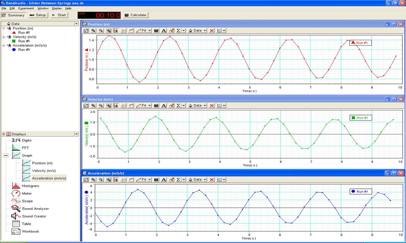
Here is a vivid, real-time demonstration of the kinematics of simple harmonic motion. The position, velocity, and acceleration are given by:
$$x(t) = A \cos (\omega t + \phi) $$
$$\nu(t) = -A \omega \sin(\omega t + \phi)$$
$$a(t) = A \omega^2 \cos (\omega t + \phi)$$
where $A =$ displacement, $\omega =$ angular frequency, and $\phi =$ phase constant.
The above graphs show these relationships between the position and its two time derivatives.
Procedure
- Verify that the Pasco Motion Sensor is connected to the laptop and that the DataStudio software suite is open to the “Air Track Glider Between Springs” activity. Turn on the air supply.
- Press the “Start” button on the screen to begin data collection. (If the “Start” button is grayed out, unplug the motion sensor’s USB cable and plug it back into the computer.)
- Move the glider about 0.5 meters toward the motion sensor and release it. Plotting will begin when the glider reaches the 1-meter mark on the air track. (If you make a mistake, you can erase the previous data run by clicking on the “Experiment” menu and selecting “Delete Last Data Run.”)
- Notice that the glider’s position, velocity and acceleration are plotted in real-time for 10 seconds.
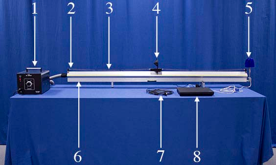
Equipment
- Air Supply
- (4) Hook Attachments
- (6) Light Springs
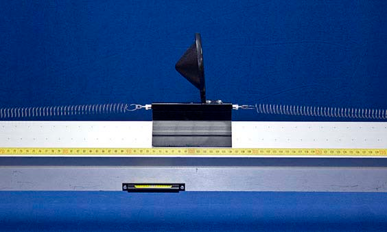
- Glider with Sonic Reflector (223g)
- Pasco Motion Sensor
- Air Track
- VGA Extension Cable
- Laptop with Pasco DataStudio